PineAPPL

Tutorial for PineAPPL’s CLI

Welcome to PineAPPL’s CLI tutorial! Here we’ll explain the basics of PineAPPL’s command-line interface (CLI): that’s the program pineappl that you can you use inside your shell to convolve grids with PDFs and to perform other operations. This tutorial will also introduce and explain the terminology needed to understand the C, Fortran, Python and Rust API.

This tutorial assumes that you understand the basics of interpolation grids. If you’d like to refresh your memory read the short overview.

Prerequisites

To follow the tutorial, you’ll first need PineAPPL’s CLI; if you haven’t installed it yet follow its installation instructions. Next, you’ll need a fresh directory. For instance, run

cd $(mktemp -d)

to create a temporary directory. Finally, you’ll need a grid,

wget 'https://data.nnpdf.science/pineappl/test-data/LHCB_WP_7TEV.pineappl.lz4'

which you’ll use with the CLI.

`pineappl convolve`: Performing convolutions

Now that you’ve got a grid, you can perform a convolution with a PDF set:

pineappl convolve LHCB_WP_7TEV.pineappl.lz4 CT18NNLO

We chose to use the default CT18 PDF set for this tutorial, because it’s the shortest to type. If you get an error that reads

error: Invalid value for '<PDFSETS>...': The PDF set `CT18NNLO` was not found

install the PDF set with LHAPDF, or use a different PDF set—the numbers won’t matter for the sake of the tutorial. If the command was successful, you should see the following output:

b   etal    dsig/detal
     []        [pb]
-+----+----+-----------
  2 2.25 7.7526895e2
2.25  2.5 7.1092145e2
2.5 2.75 6.1876958e2
2.75    3 5.0017809e2
  3 3.25 3.7228440e2
3.25  3.5 2.5236943e2
3.5    4 1.1857770e2
  4  4.5 2.7740964e1

Let’s have a closer look at what the output shows:

the b column shows there are 8 bins, indexed 0 through 7,
the next two columns labelled etal shows the observable used to define the bins and its left and right bin limits,
the last column dsig/detal shows the differential cross section (dsig) for the bin limits given in the previous two columns.

`pineappl -h`: Getting help

One of the most difficult aspects of learning a new program is remembering how to achieve certain tasks and what to type. This should be easy with pineappl; just remember that you can type

pineappl

which is a shortcut for pineappl -h. This will give you a list of program options and subcommands, under which all operations in pineappl are grouped, and a corresponding description. You’ll be familiar with the concept of subcommand if you’re using git: add, commit and push are well-known subcommands of it.

To get more help on a specific subcommand, for instance convolve, which we’ve used already, run

pineappl convolve -h

Depending on the version of PineAPPL this will show output similar to the following:

Convolutes a PineAPPL grid with a PDF set

Usage: pineappl convolve [OPTIONS] <INPUT> <PDFSETS>...

Arguments:
  <INPUT>       Path of the input grid
  <PDFSETS>...  LHAPDF id(s) or name of the PDF set(s)

Options:
  -b, --bins <BINS>       Selects a subset of bins
  -i, --integrated        Show integrated numbers (without bin widths) instead of differential ones
  -o, --orders <ORDERS>   Select orders manually
      --digits-abs <ABS>  Set the number of fractional digits shown for absolute numbers [default: 7]
      --digits-rel <REL>  Set the number of fractional digits shown for relative numbers [default: 2]
  -h, --help              Print help

This explains that pineappl convolve needs at least two arguments, the first being the grid file, denoted as <INPUT> and a second argument <PDFSETS>, which determines the PDF set. Note that this argument has three dots, ..., meaning that you’re allowed to pass multiple PDF sets, in which case pineappl will perform the convolution with each PDF set, such that you can compare them with each other. This subcommand also accepts a few optional parameters, denoted with [OPTIONS].

`pineappl read`: What does this grid contain?

If you’re experienced enough in high-energy physics, you’ve already inferred from the file name of the grid and the observable name etal what the numbers will most likely show. However, how can you be certain? Specifically, if you didn’t generate the grid yourself you’ll probably want to know the answers to the following questions:

For which process is the prediction for?
Which observable is shown?
If there’s a corresponding experimental paper, where is it?
Where are the measured values corresponding to the shown predictions?
Which program/generator was used to produce this grid? What version?
Which runcards were used, which parameter values?

The subcommand that’ll answer all questions is read. It gives you access to what we call metadata (the data describing the interpolation grids):

pineappl read --show LHCB_WP_7TEV.pineappl.lz4

This will print out a very long list of (alphabetically sorted) key–value pairs, from which you can read off the answers to the questions above. Let’s go through them one by one:

The value for the key description gives a short description of the process. In this case this is LHCb differential W-boson production cross section at 7 TeV.
The keys x1_label contains the name of the observable, and y_label the name of the corresponding (differential) cross section. These strings are being used by convolve and other subcommands that perform convolutions to label the columns with the corresponding numbers. If grids contain two- or even higher-dimensional distributions there would be additional labels, for instance x2_label, etc. Furthermore, for plots there are the corresponding labels in LaTeX: x1_label_tex, y_label_tex and so on. Finally, x1_unit contains the physical units for each observable, typically GeV, and y_unit the units of the (differential) cross section, typically in pb.
The value of the key arxiv gives us the corresponding arXiv identifier, in this case for the experimental measurement; enter the value into the search field of https://arxiv.org, and it’ll lead you to the paper.
The measured data itself you can get from the location specified by hepdata, which is a digital object identifier (DOI). Go to https://www.doi.org/ and enter the string there. This will get you to the right table on https://www.hepdata.net for the corresponding observable. Together with the paper this will make clear that the predictions show the pseudorapidity of the positively-charged lepton, corresponding to table 6 in the paper.
The presence of mg5amc_repo and mg5amc_revno show that Madgraph5_aMC@NLO was used to calculate the predictions. Since their values are empty, an official release was used, whose version we can read off from runcard. If these values were non-zero, they’d point to the Madgraph5 repository and its revision number.
Finally, the value of runcard contains runcards of the calculation and also the information that Madgraph5_aMC@NLO v3.1.0 was used run the calculation, the values of all independent parameters and a few cuts.

If you’d like a complete description of all recognized metadata, have a look at the full list.

Orders, bins and channels

Each grid is—basically—a three-dimensional array of subgrids, which are the actual interpolation grids. The three dimensions are:

orders (o),
bins (b) and
channels (c).

You can use the subcommand read to see exactly how each grid is built. Let’s go through them one by one using our grid:

pineappl read --orders LHCB_WP_7TEV.pineappl.lz4

The output is:

o      order
-+----------------
O(a^2)
O(as^1 a^2)
O(as^1 a^2 lr^1)
O(as^1 a^2 lf^1)
O(a^3)
O(a^3 lr^1)
O(a^3 lf^1)

This shows that the grid contains:

a leading order (LO) with index 0, which has the coupling alpha squared (a^2),
the QCD next-to-leading order (NLO) with index 1 and
the EW NLO with index 4.

Additionally, there are

NLO grids with factorization-log dependent terms, with indices 3 and 6. The corresponding
renormalization-logs (2 and 5) are also present, but their contributions are in fact zero.

These last two subgrid types are needed if during the convolution the scale-variation uncertainty should be calculated.

Now let’s look at the bins:

pineappl read --bins LHCB_WP_7TEV.pineappl.lz4

which prints:

b   etal    norm
-+----+----+----
  2 2.25 0.25
2.25  2.5 0.25
2.5 2.75 0.25
2.75    3 0.25
  3 3.25 0.25
3.25  3.5 0.25
3.5    4  0.5
  4  4.5  0.5

this shows the bin indices b for the observable etal, with their left and right bin limits, which you’ve already seen in convolve. The column norm shows the factor that all convolutions are divided with. Typically, as shown in this case, this is the bin width, but in general this can be different.

Finally, let’s have a look at the channel definition:

pineappl read --channels LHCB_WP_7TEV.pineappl.lz4

This prints all partonic initial states that contribute to this process:

c    entry        entry
-+------------+------------
1 × ( 2, -1) 1 × ( 4, -3)
1 × (21, -3) 1 × (21, -1)
1 × (22, -3) 1 × (22, -1)
1 × ( 2, 21) 1 × ( 4, 21)
1 × ( 2, 22) 1 × ( 4, 22)

In this case you see that the up–anti-down (2, -1) and charm–anti-strange (4, -3) initial states (the numbers are PDG MC IDs) are grouped together in a single channel, each with a factor of 1. In general this number can be different from 1, if the Monte Carlo decides to factor out CKM values or electric charges, for instance, to group more contributions with the same matrix elements together into a single channel. This is an optimization step, as fewer channels result in a smaller grid file.

Note that channels with the transposed initial states, for instance anti-down—up, are merged with each other, which always works if the two initial-state hadrons are the same; this is an optimization step, also to keep the size of the grid files small.

All remaining channels are the ones with a gluon, 21, or with a photon, 22.

`pineappl orders`: What’s the size of each perturbative order?

In the previous section you saw that each order is stored separately, which means you can perform convolutions separately for each order:

pineappl orders LHCB_WP_7TEV.pineappl.lz4 CT18NNLO

which prints

b   etal    dsig/detal  O(as^0 a^2) O(as^1 a^2) O(as^0 a^3)
     []        [pb]         [%]         [%]         [%]
-+----+----+-----------+-----------+-----------+-----------
  2 2.25 7.7526895e2      100.00       17.63       -1.25
2.25  2.5 7.1092145e2      100.00       17.47       -1.13
2.5 2.75 6.1876958e2      100.00       18.07       -1.04
2.75    3 5.0017809e2      100.00       18.53       -0.92
  3 3.25 3.7228440e2      100.00       19.12       -0.85
3.25  3.5 2.5236943e2      100.00       19.84       -0.81
3.5    4 1.1857770e2      100.00       21.32       -0.83
  4  4.5 2.7740964e1      100.00       24.59       -1.01

By default all higher orders are shown relative to the sum of all LOs. However, this can be changed using the switches --normalize or -n, which asks for the orders you define as 100 per cent. If we’d like the numbers to be normalized to NLO QCD, we’d run

pineappl orders --normalize=a2,a2as1 LHCB_WP_7TEV.pineappl.lz4 CT18NNLO

which will show

b   etal    dsig/detal  O(as^0 a^2) O(as^1 a^2) O(as^0 a^3)
     []        [pb]         [%]         [%]         [%]
-+----+----+-----------+-----------+-----------+-----------
  2 2.25 7.7526895e2       85.01       14.99       -1.06
2.25  2.5 7.1092145e2       85.13       14.87       -0.96
2.5 2.75 6.1876958e2       84.69       15.31       -0.88
2.75    3 5.0017809e2       84.37       15.63       -0.78
  3 3.25 3.7228440e2       83.95       16.05       -0.71
3.25  3.5 2.5236943e2       83.45       16.55       -0.67
3.5    4 1.1857770e2       82.42       17.58       -0.69
  4  4.5 2.7740964e1       80.26       19.74       -0.81

`pineappl channels`: What’s the size of each channel?

You can also show a convolution separately for each channel:

pineappl channels LHCB_WP_7TEV.pineappl.lz4 CT18NNLO

This will show the following table,

b   etal    c  size  c  size  c size  c size c size
     []        [%]      [%]      [%]    [%]    [%]
-+----+----+-+------+-+------+-+-----+-+----+-+----
  2 2.25 0 111.00 3  -7.91 1 -3.10 2 0.00 4 0.00
2.25  2.5 0 111.83 3  -8.69 1 -3.15 2 0.00 4 0.00
2.5 2.75 0 112.68 3  -9.37 1 -3.31 2 0.00 4 0.00
2.75    3 0 113.49 3  -9.97 1 -3.53 2 0.00 4 0.00
  3 3.25 0 114.26 3 -10.36 1 -3.90 2 0.00 4 0.00
3.25  3.5 0 115.00 3 -10.58 1 -4.42 2 0.00 4 0.00
3.5    4 0 115.65 3 -10.25 1 -5.39 2 0.00 4 0.00
  4  4.5 0 115.81 3  -8.58 1 -7.23 2 0.00 4 0.00

The most important channel is 0, which is the up-type–anti-down-type combination. The channels with gluons are much smaller and negative. Channels with a photon are zero, because the PDF set that we’ve chosen doesn’t have a photon PDF. Let’s try again with NNPDF31_nnlo_as_0118_luxqed (remember to install the set first) as the PDF set:

b   etal    c  size  c  size  c size  c size c size
     []        [%]      [%]      [%]    [%]    [%]
-+----+----+-+------+-+------+-+-----+-+----+-+----
  2 2.25 0 111.04 3  -7.84 1 -3.23 4 0.02 2 0.01
2.25  2.5 0 111.87 3  -8.62 1 -3.29 4 0.02 2 0.01
2.5 2.75 0 112.73 3  -9.31 1 -3.45 4 0.02 2 0.01
2.75    3 0 113.56 3  -9.90 1 -3.69 4 0.01 2 0.01
  3 3.25 0 114.34 3 -10.30 1 -4.07 4 0.01 2 0.01
3.25  3.5 0 115.07 3 -10.52 1 -4.57 4 0.02 2 0.01
3.5    4 0 115.59 3 -10.18 1 -5.43 2 0.01 4 0.01
  4  4.5 0 115.16 3  -8.23 1 -6.94 4 0.01 2 0.01

`pineappl uncert`: How large are the scale and PDF uncertainties?

Let’s calculate the scale and PDF uncertainties for our grid:

pineappl uncert --pdf --scale-env=7 LHCB_WP_7TEV.pineappl.lz4 NNPDF31_nnlo_as_0118_luxqed

This will show a table very similar to pineappl convolve:

b   etal    dsig/detal  PDF central    PDF     7pt-svar (env)
     []        [pb]                    [%]           [%]
-+----+----+-----------+-----------+-----+----+-------+-------
  2 2.25 7.7651327e2 7.7650499e2 -1.01 1.01   -3.69    2.64
2.25  2.5 7.1011428e2 7.1008027e2 -1.01 1.01   -3.67    2.69
2.5 2.75 6.1683947e2 6.1679433e2 -1.01 1.01   -3.67    2.76
2.75    3 4.9791036e2 4.9786461e2 -1.03 1.03   -3.64    2.78
  3 3.25 3.7016249e2 3.7012355e2 -1.07 1.07   -3.60    2.80
3.25  3.5 2.5055318e2 2.5052366e2 -1.13 1.13   -3.55    2.81
3.5    4 1.1746882e2 1.1745148e2 -1.33 1.33   -3.48    2.80
  4  4.5 2.8023753e1 2.8018010e1 -4.05 4.05   -3.40    2.74

The first three columns are exactly the one that pineappl convolve shows. The next columns are the PDF central predictions, and negative and positive PDF uncertainties. These uncertainties are calculated using LHAPDF, so pineappl always uses the correct algorithm no matter what type of PDF sets you use: Hessian, Monte Carlo, etc. Note that we’ve chosen a PDF set with Monte Carlo replicas which means that the results shown in dsig/detal and PDF central aren’t exactly the same. The first number is calculated from the zeroth replica of the set and the second number is the average of all replicas (except the zeroth). You’ll notice that the PDF uncertainties are symmetric, which will not necessarily be the case with Hessian PDF sets, for instance.

The two remaining columns show the scale-variation uncertainty which is estimated from taking the envelope of a 7-point scale variation. By changing the parameter of --scale-env to a different value (3 or 9), you can change the scale-variation procedure.

`pineappl pull`: Are two PDF sets compatible with each other?

A variation of PDF uncertainties are pulls; they quantify how different predictions for two PDF sets are. The pull is defined as the difference of the two predictions $\sigma_1$ and $\sigma_2$, in terms of their PDF uncertainties $\delta \sigma_1$ and $\delta \sigma_2$:

\[\text{pull} = \frac{\sigma_2 - \sigma_1}{\sqrt{(\delta \sigma_1)^2 + (\delta \sigma_2)^2}}\]

You can calculate it for each bin using:

pineappl pull LHCB_WP_7TEV.pineappl.lz4 CT18NNLO NNPDF31_nnlo_as_0118_luxqed

in which CT18NNLO will be used to calculate $\sigma_1$ and $\delta \sigma_1$ and NNPDF31_nnlo_as_0118_luxqed for $\sigma_2$ and $\delta \sigma_2$. This will show not only the pull, in the column total, but also how this pull is calculated using the different channels:

b   etal    total  c  pull  c  pull  c  pull  c pull  c pull
     []      [σ]      [σ]      [σ]      [σ]      [σ]     [σ]
-+----+----+------+-+------+-+------+-+------+-+-----+-+-----
  2 2.25  0.065 0  0.086 1 -0.058 3  0.024 4 0.009 2 0.005
2.25  2.5 -0.037 1 -0.042 0 -0.029 3  0.024 4 0.006 2 0.004
2.5 2.75 -0.102 0 -0.097 1 -0.043 3  0.030 4 0.006 2 0.002
2.75    3 -0.149 0 -0.148 1 -0.045 3  0.036 4 0.005 2 0.004
  3 3.25 -0.188 0 -0.190 1 -0.045 3  0.039 4 0.004 2 0.003
3.25  3.5 -0.235 0 -0.250 3  0.044 1 -0.037 4 0.005 2 0.002
3.5    4 -0.283 0 -0.344 3  0.050 1  0.004 2 0.003 4 0.003
  4  4.5  0.144 0  0.073 3  0.037 1  0.031 4 0.002 2 0.001

Looking at the total column you can see that the numbers are much smaller than 1, where 1 corresponds to a one sigma difference. This we expect knowing that this dataset is used in the fit of both PDF sets. The remaining columns show how different channels (with indices in the c column) contribute to the total pull. For the last bin, for instance, we see channel 0 contributes roughly half to the total pull, the remaining pull coming from channels 3 and 1.

Note that CT18NNLO doesn’t have a photon PDF, but the NNPDF set has one. However, for these observables the photon PDF contribution is too small to make a difference in the pull.

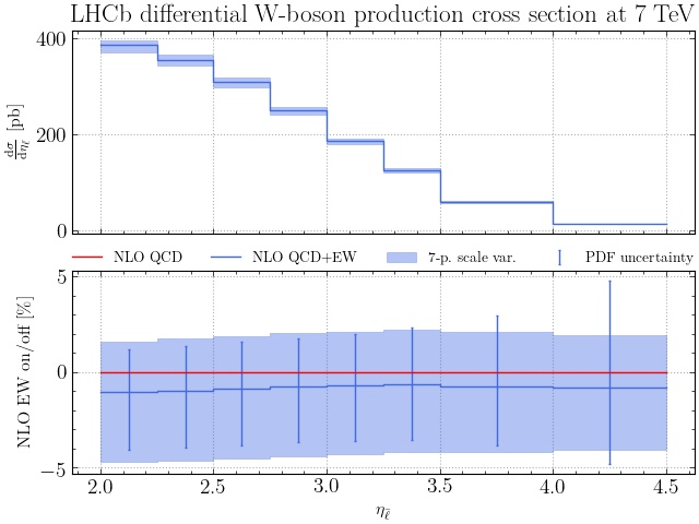
`pineappl plot`: Show me a plot of the predictions!

Often a good way to start understanding predictions is to plot them. Fortunately, this is easy with PineAPPL:

pineappl plot LHCB_WP_7TEV.pineappl.lz4 CT18NNLO > plot.py

This will write a matplotlib script in Python. Note that the script is written to the standard output and redirected into plot.py. The advantage of writing a plotting script instead of directly producing the plot is that you can change it according to your needs. Finally, let’s run the plotting script:

python3 plot.py

This will create the file LHCB_WP_7TEV.pdf, which you can open. If you need a different format than .pdf, look for the string '.pdf' in the plotting script and change it to the file ending corresponding to your desired format. Here’s how the result for .jpeg looks:

plot

The plot subcommand is much more powerful, however. It accepts multiple PDF sets, for instance

pineappl plot LHCB_WP_7TEV.pineappl.lz4 NNPDF31_nnlo_as_0118_luxqed=NNPDF31luxQED \
    CT18NNLO=CT18 MSHT20nnlo_as118=MSHT20 > plot.py

in which case more insets are plotted, which show the PDF uncertainty for each set and also the pull using the first PDF set. As shown above, you can use =plotlabel after the LHAPDF name to change the labels in the plot:

plot

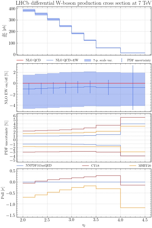
Note that you easily customize the generated script, plot.py in this case. It is generated in such a way that style choices, plot labels and panel selection is at the top of the script and separated from plotting routines and data, which are found at the end of the file.

Conclusion

This is the end of the tutorial, but there are many more subcommands left that we didn’t discuss, and many more switches for subcommands that weren’t part of the tutorial. Remember that you can always run

pineappl

to get an overview of what’s there and what you might need, and that

pineappl <SUBCOMMAND> -h

gives you a more detailed description of the options and switches for each subcommand.

This site is open source. Improve this page.

PineAPPL

Tutorial for PineAPPL’s CLI

Prerequisites

pineappl convolve: Performing convolutions

pineappl -h: Getting help

pineappl read: What does this grid contain?

Orders, bins and channels

pineappl orders: What’s the size of each perturbative order?

pineappl channels: What’s the size of each channel?

pineappl uncert: How large are the scale and PDF uncertainties?

pineappl pull: Are two PDF sets compatible with each other?

pineappl plot: Show me a plot of the predictions!